Fastq Utilities

Determining/Improving Read Quality

FASTQ is a text-based format for storing both a nucleotide sequence and its corresponding quality scores. Both the sequence letter and quality score are each encoded with a single ASCII character.

A FASTQ file normally uses four lines per sequence.

• Line 1 begins with a ‘@’ character and is followed by a sequence identifier and an optional description (like a FASTA title line).

• Line 2 is the raw sequence letters.

• Line 3 begins with a ‘+’ character and is optionally followed by the same sequence identifier (and any description) again.

• Line 4 encodes the quality values for the sequence in Line 2, and must contain the same number of symbols as letters in the sequence.

Understanding the quality of fastq reads that come from the sequencer is an essential first step to any of the PATRIC services that uses them (Assembly, Comprehensive Genome Analysis, Taxonomic classification, Metagenomic read mapping, Metagenomic binning, Variation, RNA-Seq, TN-seq and Similar Genome Finder). The Fastq Utilities Service provides the capability for aligning, measuring base call quality, and trimming fastq read files to estimate quality. Researchers can submit fastq reads (paired-or single-end, long or short, zipped or not) to the service, as well as Sequence Read Archive accession numbers. The three components (trim, fastqc and align) can be used independently, or in any combination.

Locating The Fastq Utilities Service App

1. At the top of any PATRIC page, find the Services tab and click on it

2. In the drop-down box, underneath Data, click on Fastq Utilities.

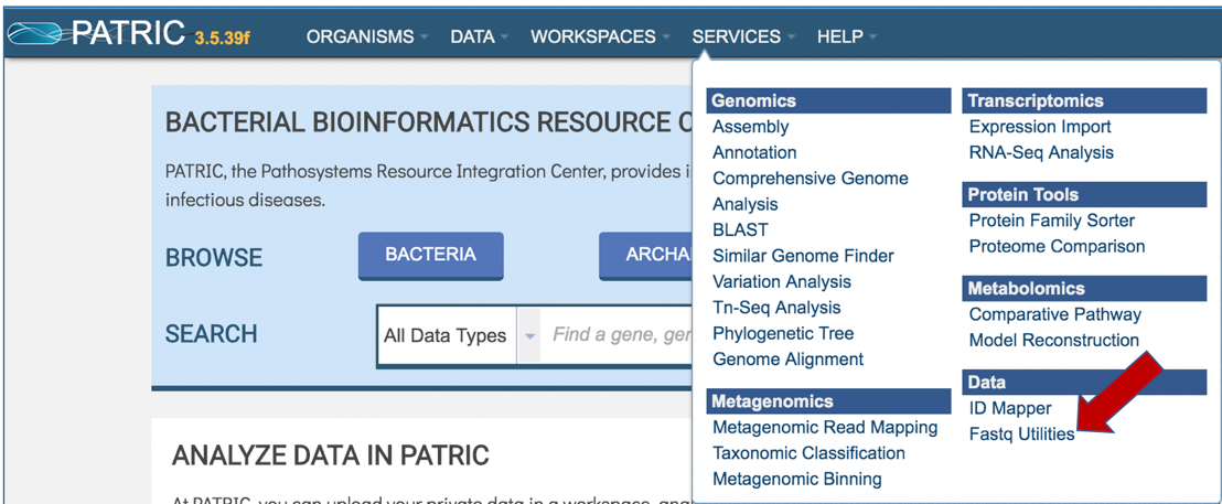
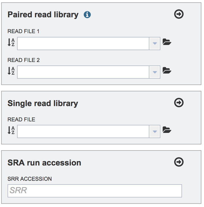
3. This will open up the Fastq Utilities landing page where researchers can submit single or paired read files, an SRA run accession number to the service.

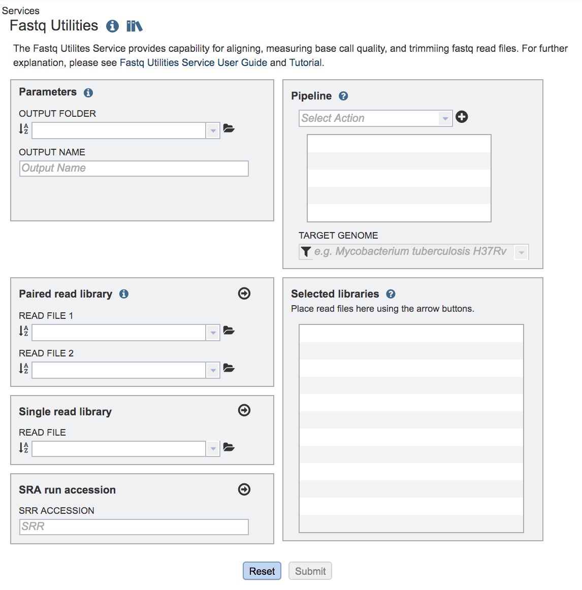
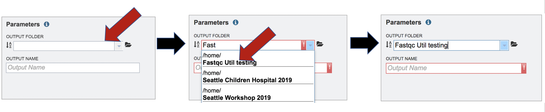
4. A folder must be selected for the Fastqc Utilities job. Clicking on the down arrow at the end of the text box underneath Output Folder will show recent folders that have been used. Clicking on the folder icon at the end of the text box will open a pop-up window where all folders can be viewed, or new folders created.

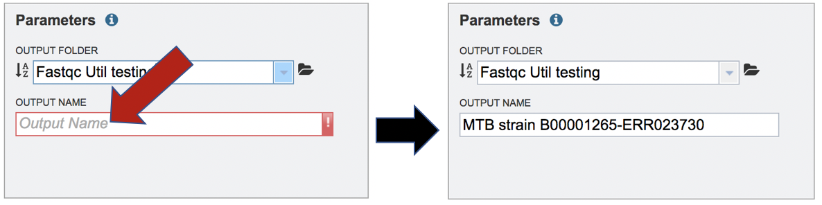
5. A name for the job must be entered in the text box under Output Name.

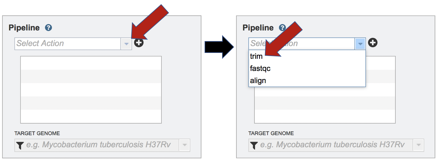
6. The Fastq Utilities service allows researchers to judge the quality of their reads, trim them, or align them to a reference genome. Each of these steps, which can be launched independently or in any combination, will be described below, To select the type of pipeline, click on the down-arrow at the end of the text box that says Select Action. This will open a drop-down box that shows the three available pipelines. Click on pipeline of choice.

Trimming Fastq Reads

The lengths of individual nucleotide sequences (reads) output by second-generation sequencing machines have reached 35, 50, 100 bps and more. When DNA or RNA molecules are sequenced that are shorter than this length the machine sequences into the adapter ligated to the 3 end of each molecule during library preparation. Consequently, the reads contain the sequence of the molecule of interest and also the adapter sequence. An essential first task prior to analysis is to find the reads containing adapters and to remove those adapters, leaving the relevant part of the read for downstream analysis. In some cases, finding adapters is a sign of contamination, and the reads containing them must be discarded entirely. The Trim component of Fastq Utilities service uses Trim Galore[1], which is Perl wrapper around the Cutadapt[2] and FastQC[3] tools. The Trim Galore algorithm was downloaded from the following source: https://github.com/FelixKrueger/TrimGalore

Uploading Paired End Reads

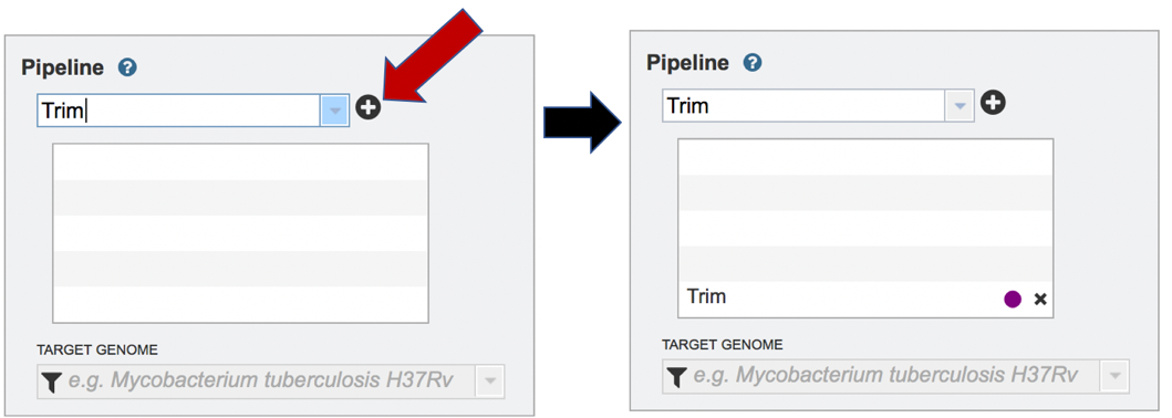
1. Clicking on trim in the drop-down box will move it into the text box. Click on the plus icon (+) at the end of the text box to move that pipeline into the selected service box below.

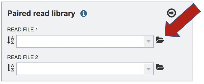
2. To upload a fastq file that contains paired reads, locate the box called Paired read library.

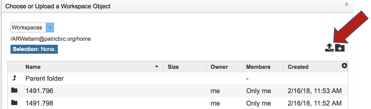
3. The reads must be located in the workspace. To initiate the upload, first click on the folder icon.

4. This opens up a window where the files for upload can be selected. Click on the icon with the arrow pointing up.

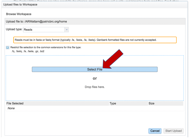
5. This opens a new window where the file you want to upload can be selected. Click on the Select File in the blue bar.

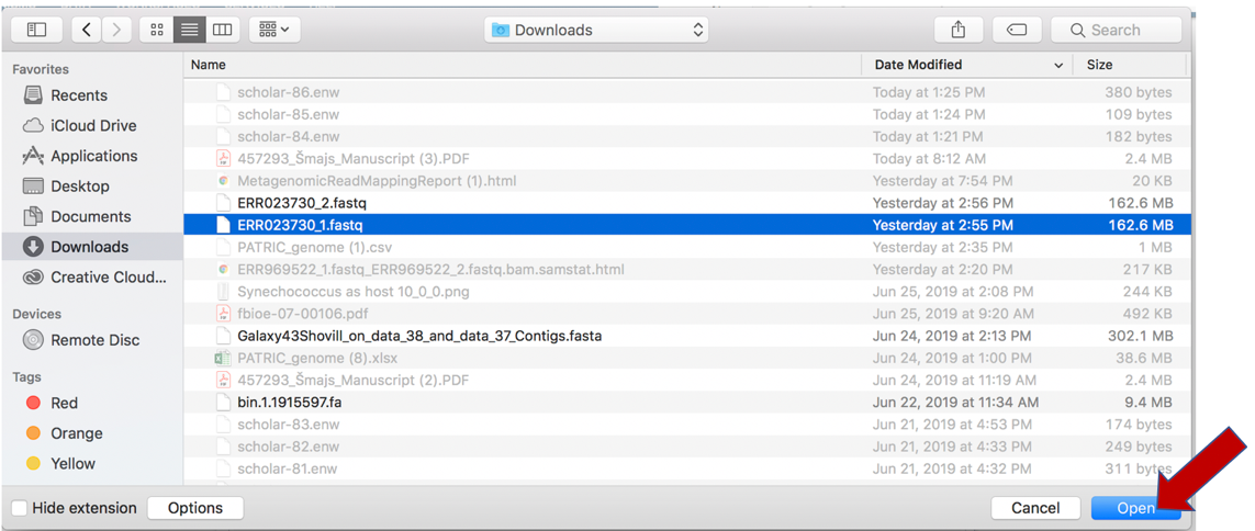
6. This will open a window that allows you to choose files that are stored on your computer. Select the file where you stored the fastq file on your computer and click Open.

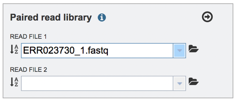
7. Once selected, it will autofill the name of the file. Click on the Start Upload button.

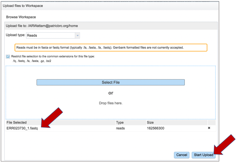
8. This will auto-fill the name of the document into the text box.

9. Pay attention to the upload monitor in the lower right corner of the PATRIC page. It will show the progress of the upload. Do not submit the job until the upload is 100% complete.

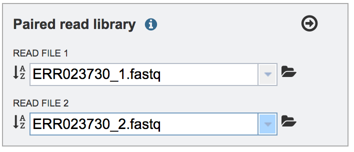
10. Repeat to upload the second pair of reads.

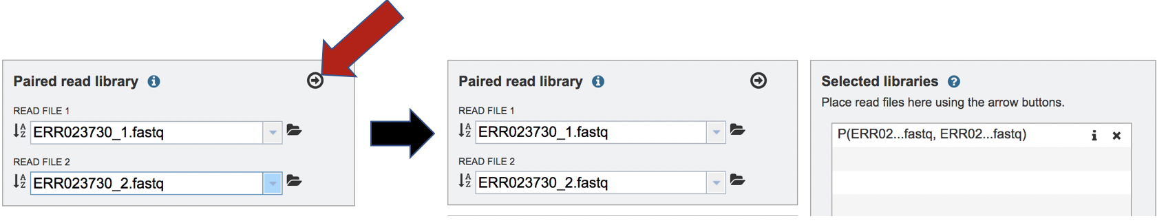
11. To finish the upload, click on the icon of an arrow within a circle. This will move your file into the Selected libraries box.

Uploading Single Reads

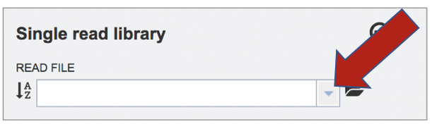
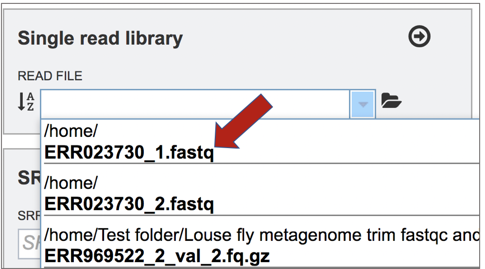
1. To upload a fastq file that contains single reads, locate the text box called �Single read library.� If the reads have previously been uploaded, click the down arrow next to the text box below Read File.

2. This opens up a drop-down box that shows the all the reads that have been previously uploaded into the user account. Click on the name of the reads of interest.

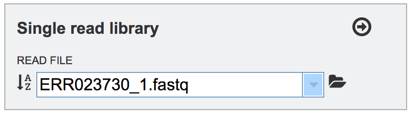
3. This will auto-fill the name of the file into the text box.

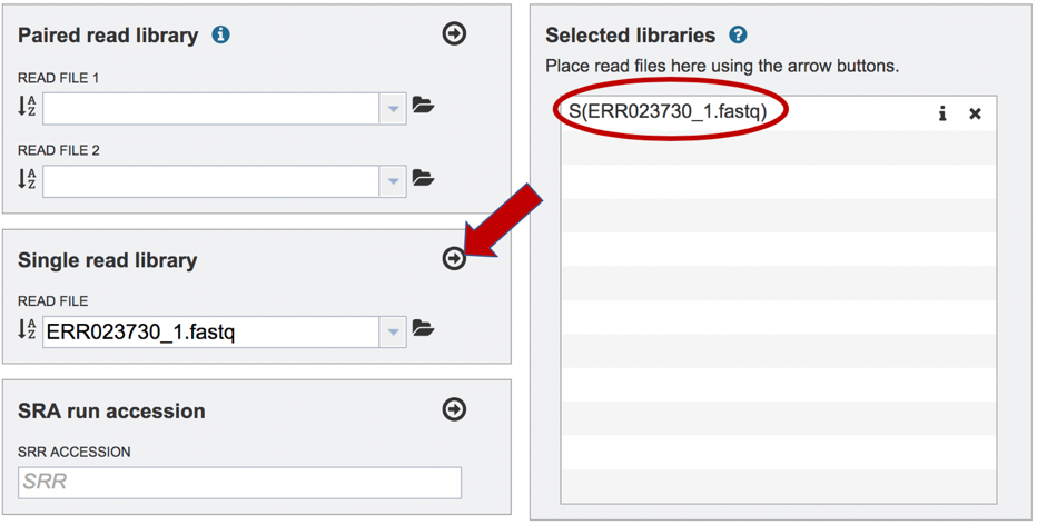
4. To finish the upload, click on the icon of an arrow within a circle. This will move the file into the Selected libraries box.

Submitting reads that are present at the Sequence Read Archive (SRA)

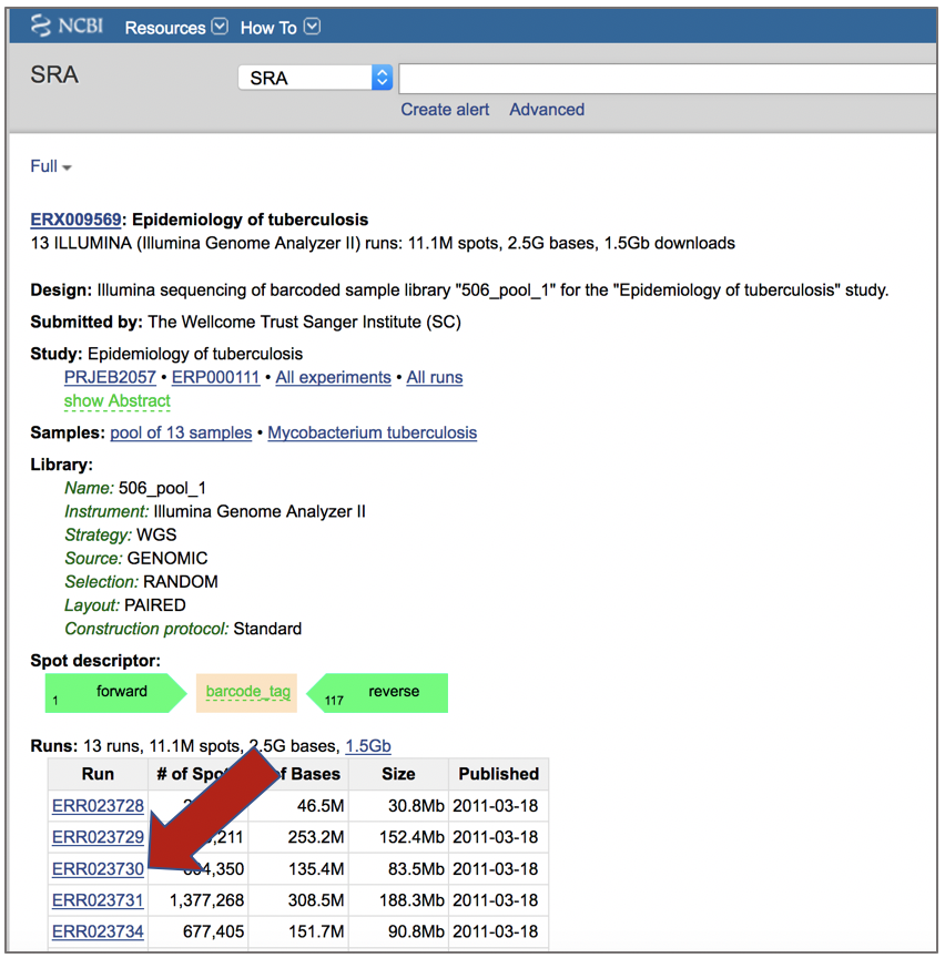
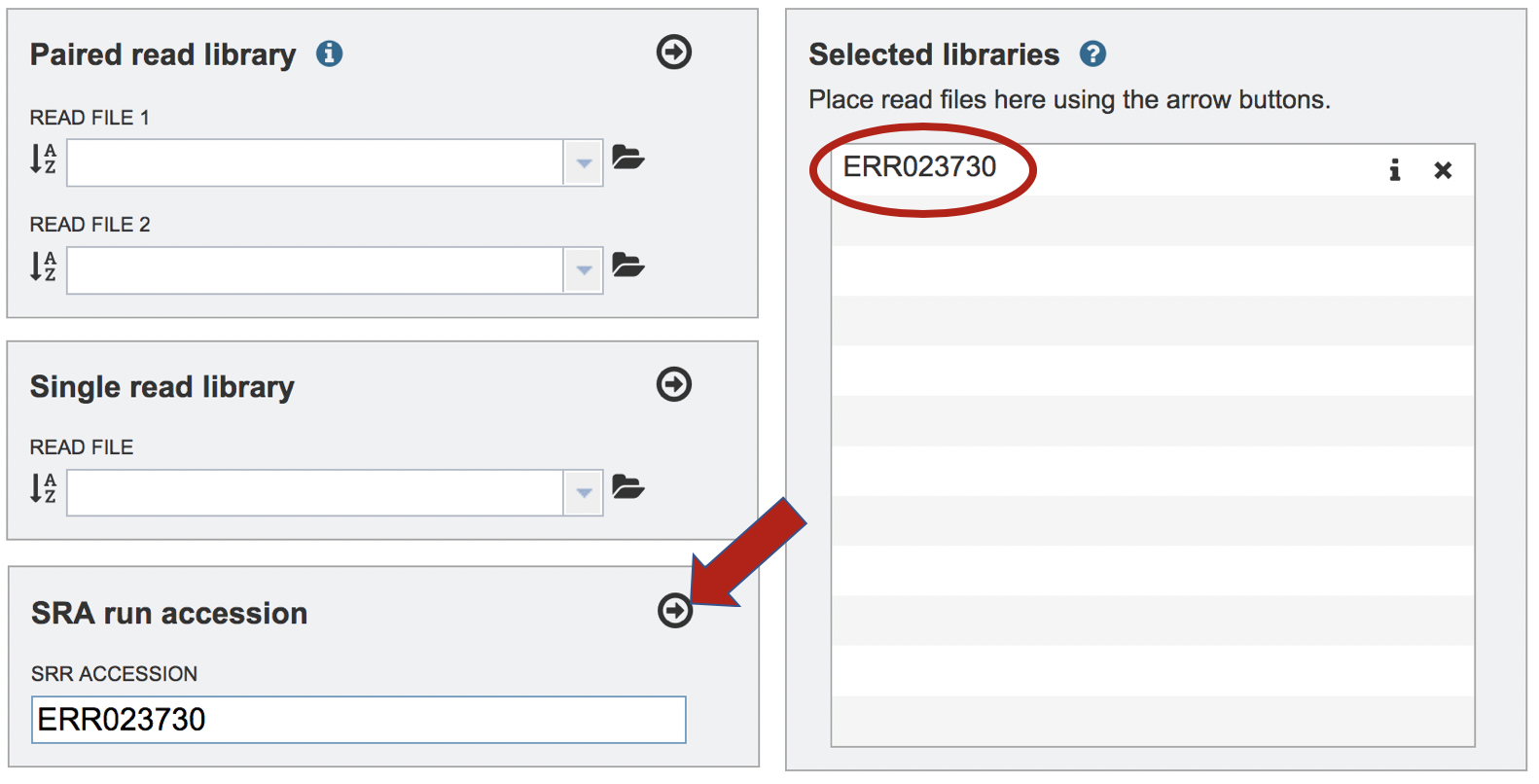
1. PATRIC also supports analysis of existing datasets from SRA. To submit this type of data, locate the Run Accession number and copy it.

2. Paste the copied accession number in the text box underneath SRA Run Accession, then click on the icon of an arrow within a circle. This will move the file into the Selected libraries box.

Submitting the job

1. Once the Parameters and Reads have been filled in or selected, the Submit button turns blue and the job will be submitted once clicked.

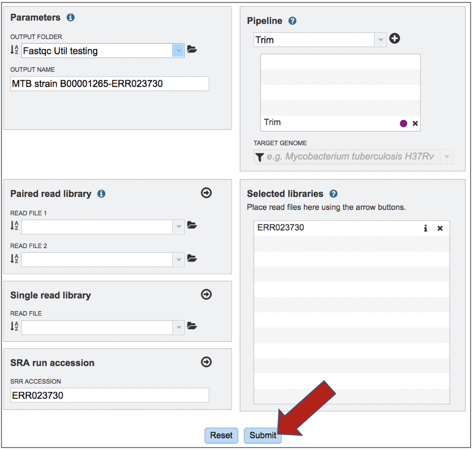
2. A successful submission will generate a message indicating that the job has been queued.

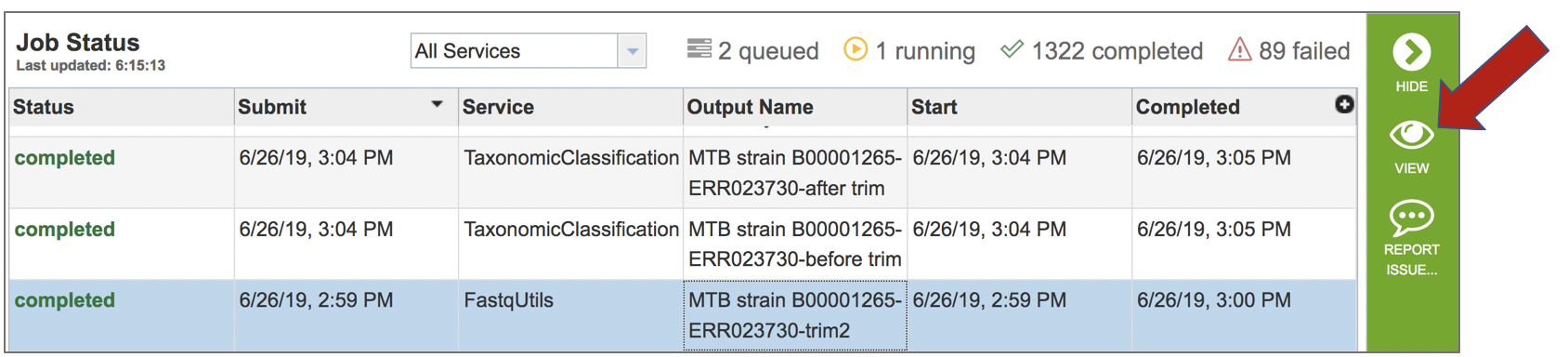
Viewing the trimming job

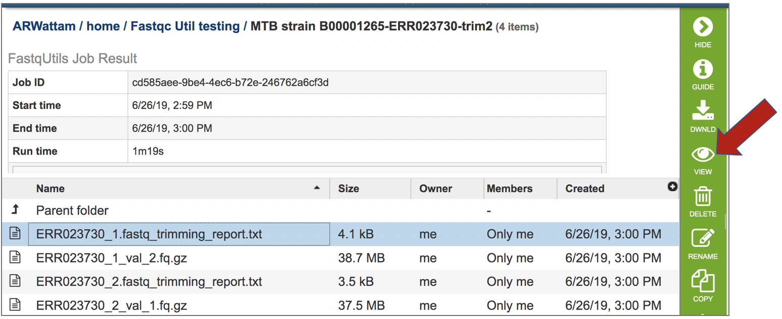
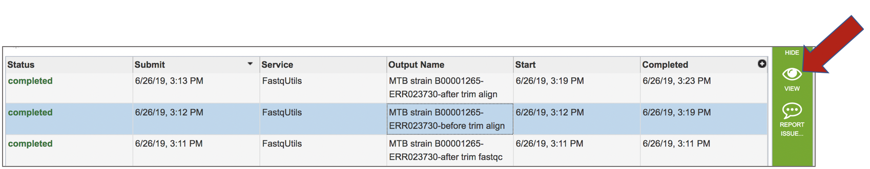
1. A job that has been successfully completed can be viewed by clicking on the row and then clicking on the View icon in the vertical green bar.

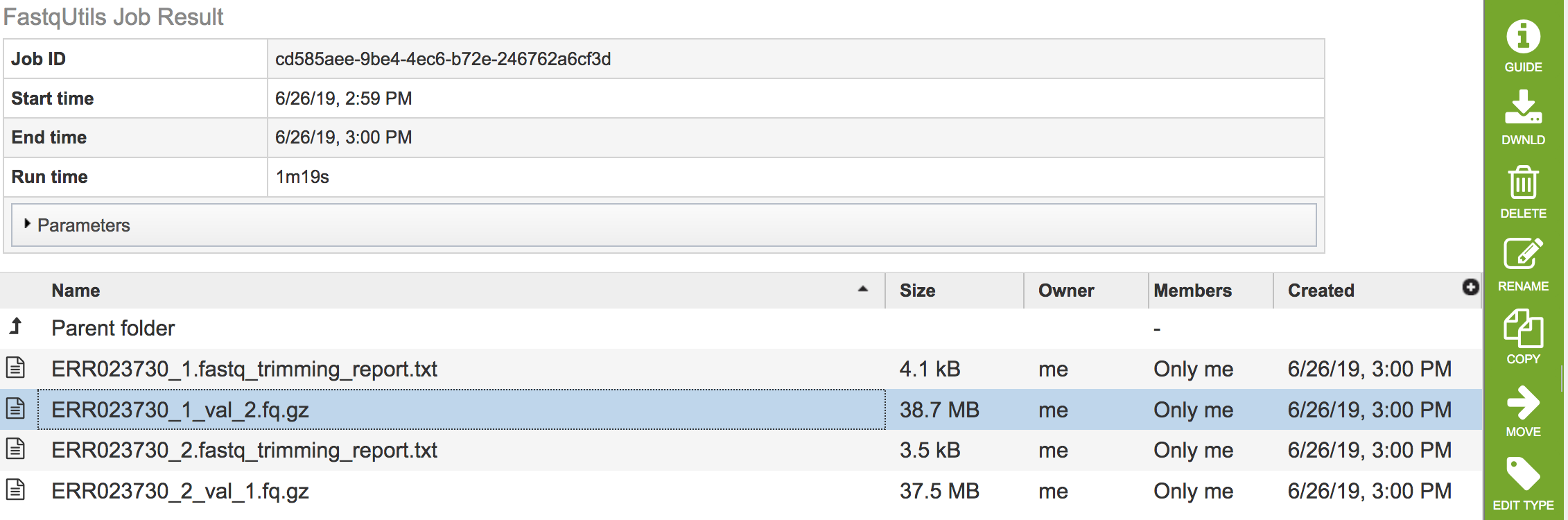
2. This will open the landing page for the selected job. The top box has the job ID number and gives pertinent information about the time it took to complete and the selected parameters. The lower table has four output files. Clicking on any of the rows that have the output files will fill the vertical green bar with the possible actions that can be taken with that file.

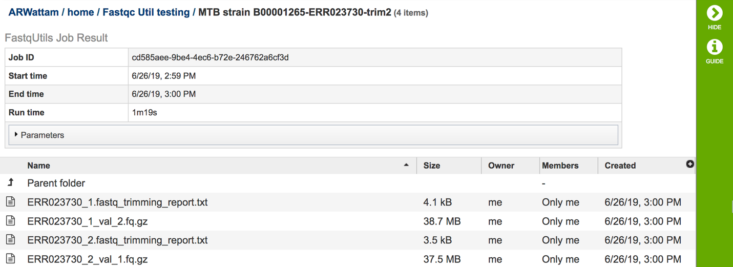
The trimming report.txt file(s)

If single reads were submitted, there will be one file. If paired reads were submitted, there will be two files (one per read file). These files include a summary of the pipeline parameters and the details on the reads that were processed.

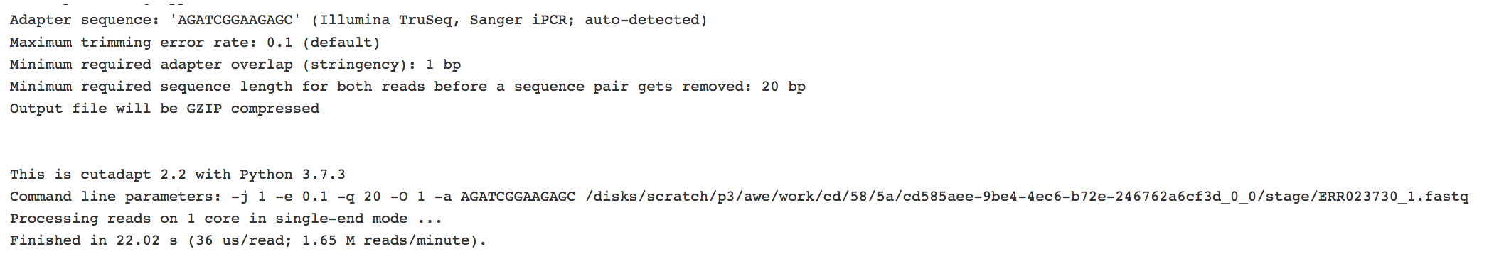
1. To view this file, click on the row then the View icon in the vertical green bar.

2. The file contains details about the default parameters used in running the pipeline, including information about any adaptor sequences that were located.

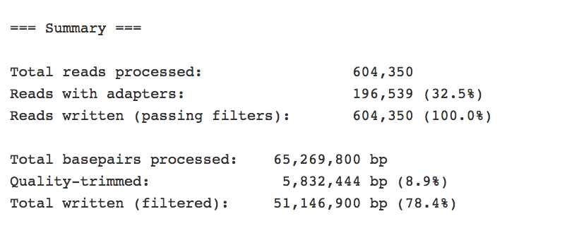
3. It provides information on the reads and base pairs processed.

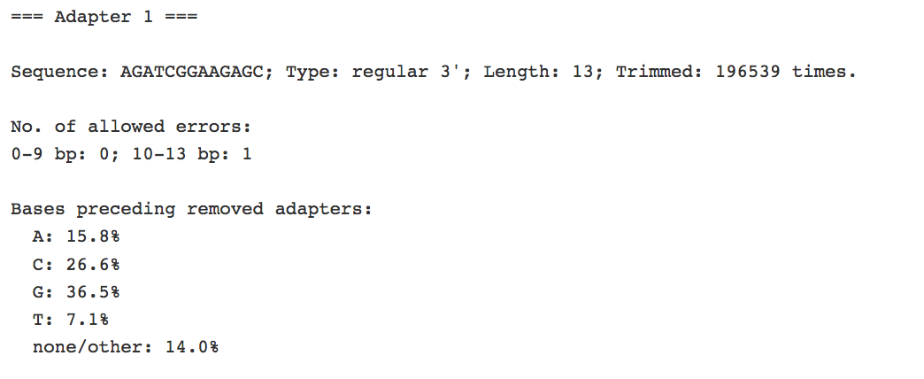
4. It provides information about any adaptors that it finds.

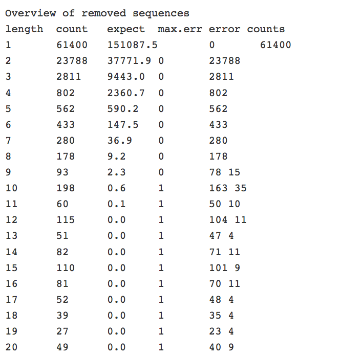
5. It contains an overview of removed sequences.

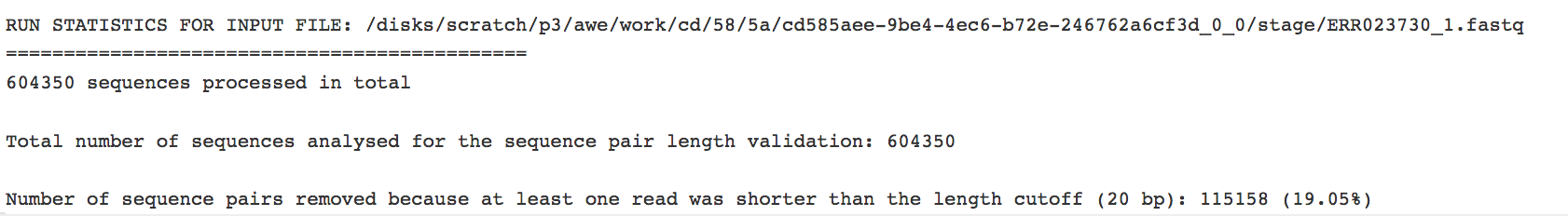
6. It also includes the run statistics for the input file, which includes the number of sequences that were removed.

Files that end in fq.gz

These files contain the trimmed read files, and should be used for downstream analyses.

Running FastQC

FastQC[3] provides a simple way to do some quality control checks on raw sequence data coming from high throughput sequencing pipelines. It provides a modular set of analyses that provide a quick impression of the data and indicate any problems that would impact further analysis. The FastQC algorithm was downloaded from Babraham Bioinformatics (http://www.bioinformatics.babraham.ac.uk/projects/fastqc/). An excellent tutorial on the FastQC report is provided by Michigan State University (https://rtsf.natsci.msu.edu/genomics/tech-notes/fastqc-tutorial-and-faq/), part of which is provided below.

Submitting the FastQC job

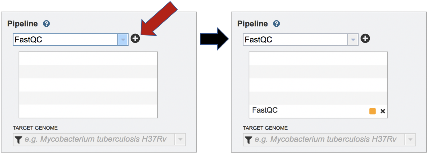
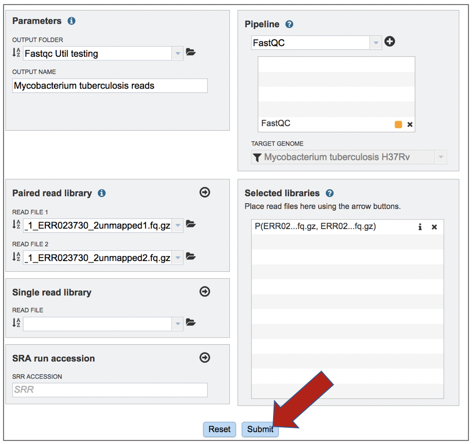
1. Clicking on FastQC in the drop-down box will move it into the text box. Click on the plus icon (+) at the end of the text box to move that pipeline into the selected service box below.

2. Uploading paired-end, single-end or reads available at the Sequence Read Archive are described above.

3. Once the Parameters and Reads have been filled in or selected, the Submit button turns blue and the job will be submitted once clicked.

Viewing the FastQC job

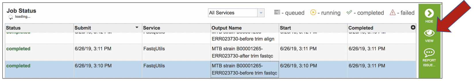
1. A job that has been successfully completed can be viewed by clicking on the row and then clicking on the View icon in the vertical green bar.

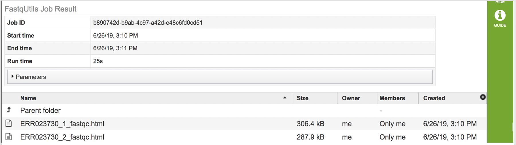
2. This will open the landing page for the selected job. The top box has the job ID number and gives pertinent information about the time it took to complete and the selected parameters. The lower table has output files (fastqc.html). If single reads were submitted, there will be one fastqc.html file, and if paired reads were submitted, there will be two. Clicking on any of the rows that have the output files will fill the vertical green bar with the possible actions that can be taken with that file.

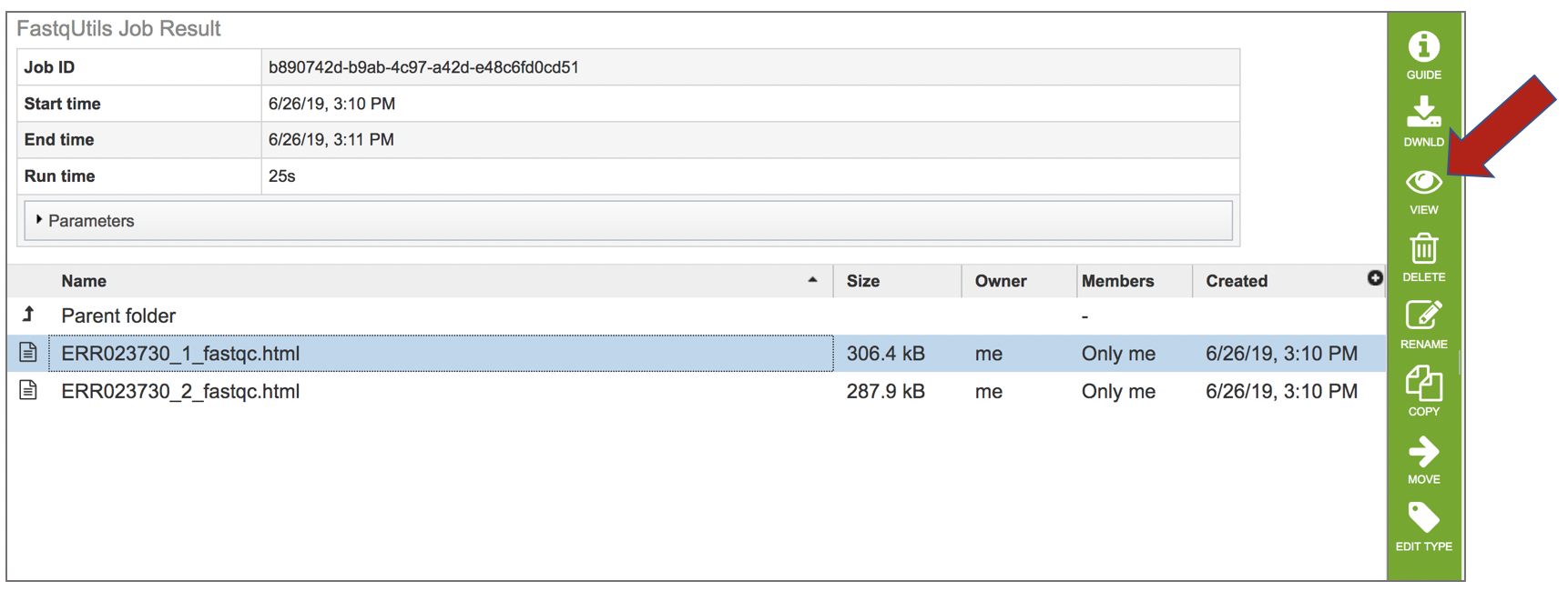
Viewing the fastqc.html report

1. To view this file, click on the row then the View icon in the vertical green bar.

2. This will open a report on the quality of the selected reads.

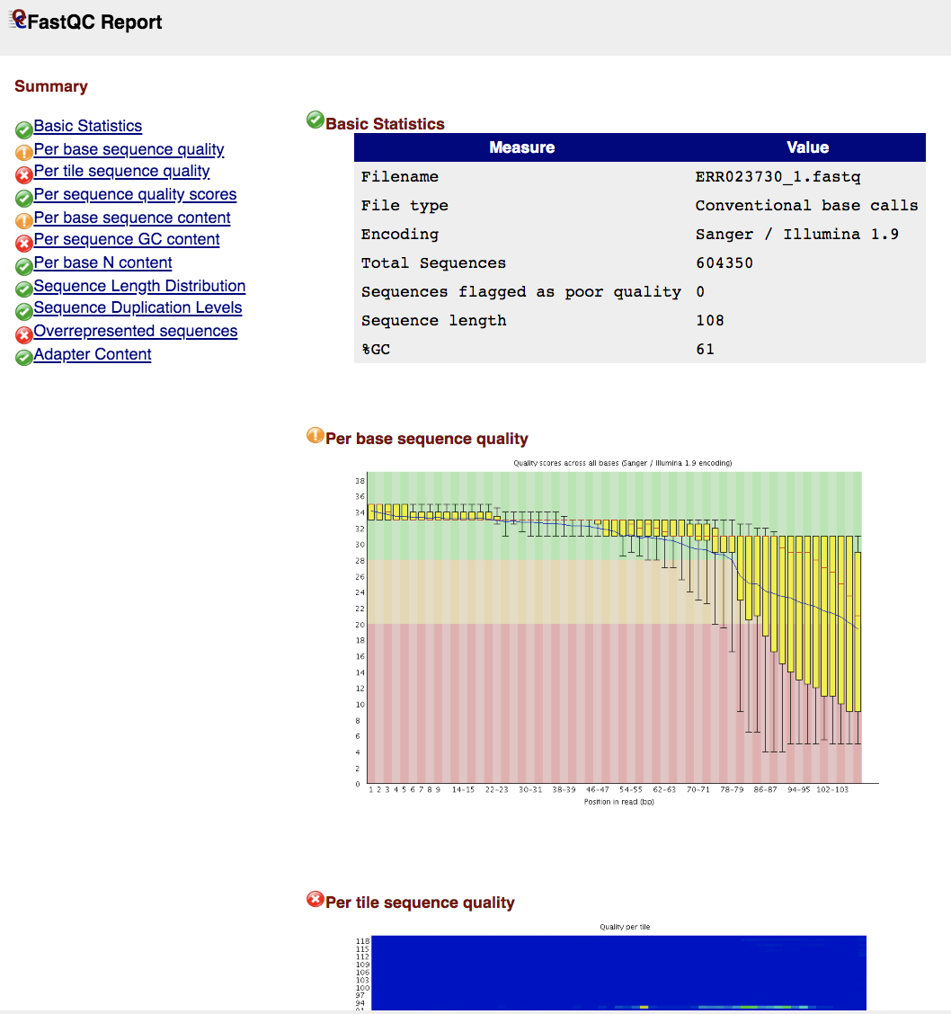
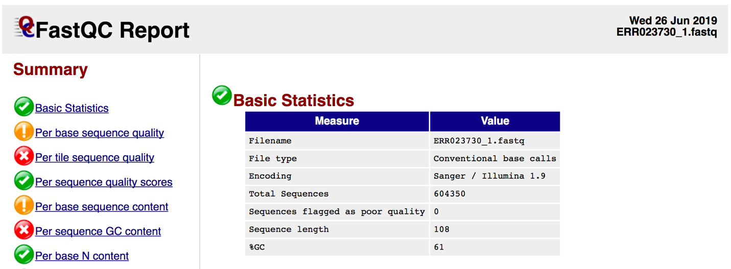
3. Basic Statistics contains information about input FASTQ file: its name, type of quality score encoding, total number of reads, reads tagged as poor quality, read length and GC content.

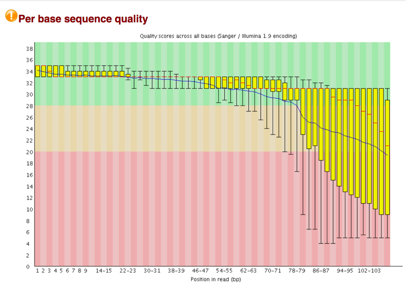
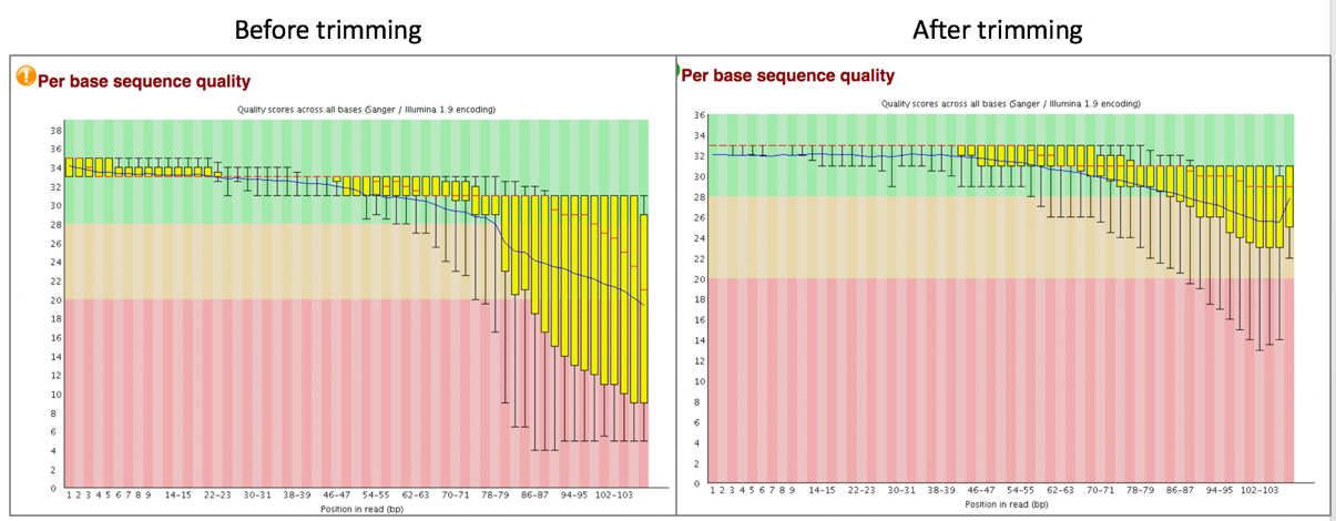
4. Per Sequence Base Quality A box-and-whisker plot showing aggregated quality score statistics at each position along all reads in the file. Note that the X-axis is not uniform, it starts out with bases 1-10 being reported individually, after that, it will bin bases across a window a certain number of positions wide. The number of base positions binned together depends on the length of the read; for example, with 150bp reads the latter part of the plot will report aggregate statistics for 5bp windows. Shorter reads will have smaller windows and longer reads larger windows. The blue line is the mean quality score at each base position/window. The red line within each yellow box represents the median quality score at that position/window. Yellow box is the inner-quartile range for 25th to 75th percentile. The upper and lower whiskers represent the 10th and 90th percentile scores. It is normal with all Illumina sequencers for the median quality score to start out lower over the first 5-7 bases and to then rise. The average quality score will steadily drop over the length of the read. With paired end reads the average quality scores for read 1 will almost always be higher than for read 2.

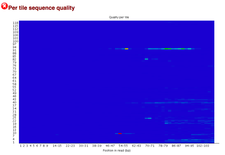
5. Per Tile Sequence Quality The plot shows the deviation from the average quality for each tile. The colors are on a cold to hot scale, with cold colors being positions where the quality was at or above the average for that base in the run, and hotter colors indicate that a tile had worse qualities than other tiles for that base. In the example below you can see that certain tiles show consistently poor quality. A good plot should be blue all over.

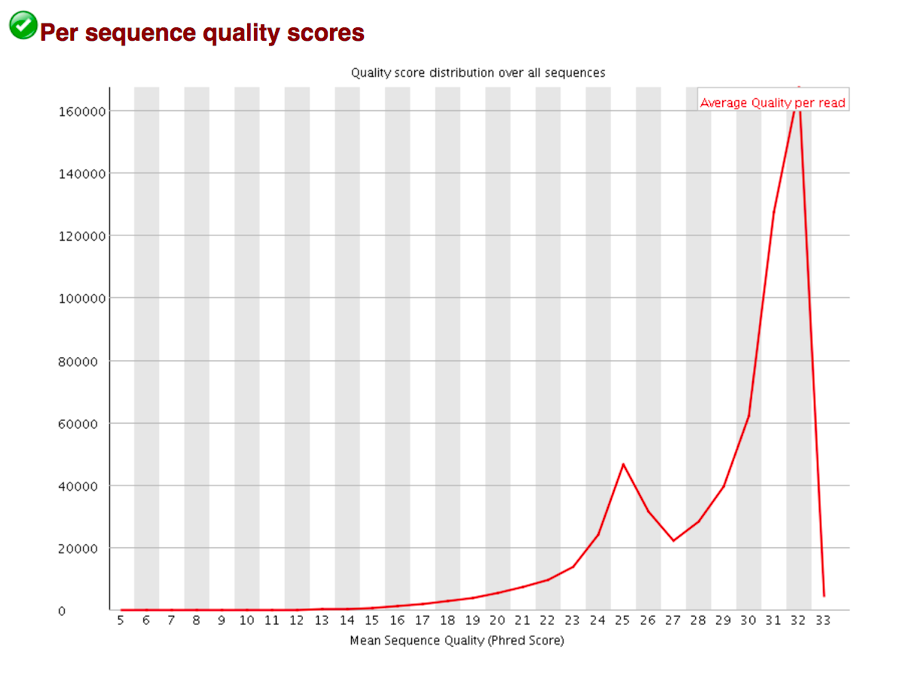
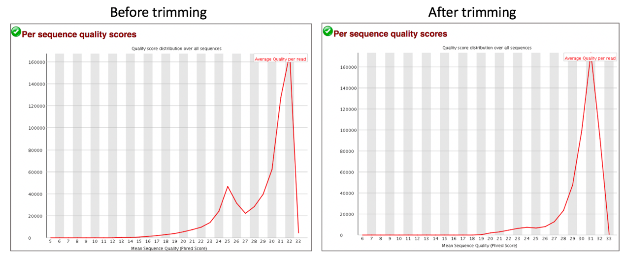
6. Per Sequence Quality Scores shows a plot of the total number of reads vs the average quality score over full length of that read. The distribution of average read quality should be fairly tight in the upper range of the plot.

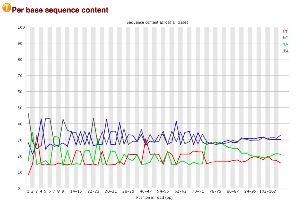
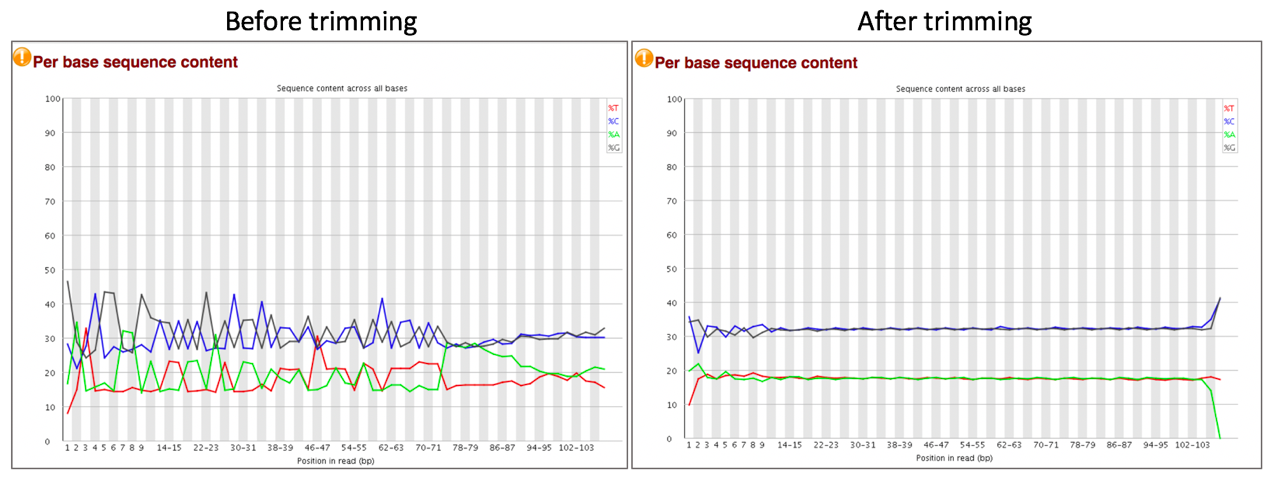
7. The Per Base Sequence Content plot reports the percent of bases called for each of the four nucleotides at each position across all reads in the file. The X-axis is non-uniform as described for Per base sequence quality.

1. For whole genome shotgun DNA sequencing the proportion of each of the four bases should remain relatively constant over the length of the read with %A=%T and %G=%C. With most RNA-Seq library preparation protocols there is clear non-uniform distribution of bases for the first 10-15 nucleotides; this is normal and expected depending on the type of library kit used (e.g. TruSeq RNA Library Preparation). RNA-Seq data showing this non-uniform base composition will always be classified as Failed by FastQC for this module even though the sequence is perfectly good.

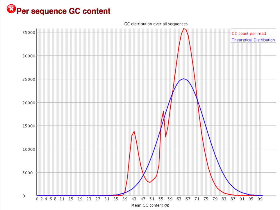
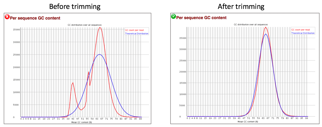
8. The Per Sequence GC Content plot shows the number of reads vs. GC% per read. The displayed Theoretical Distribution assumes a uniform GC content for all reads.

1. For whole genome shotgun sequencing the expectation is that the GC content of all reads should form a normal distribution with the peak of the curve at the mean GC content for the organism sequenced. If the observed distribution deviates too far from the theoretical, FastQC will call a Fail. There are many situations in which this may occur which are expected so the assignment can be ignored. For example, in RNA sequencing there may be a greater or lesser distribution of mean GC content among transcripts causing the observed plot to be wider or narrower than an idealized normal distribution.

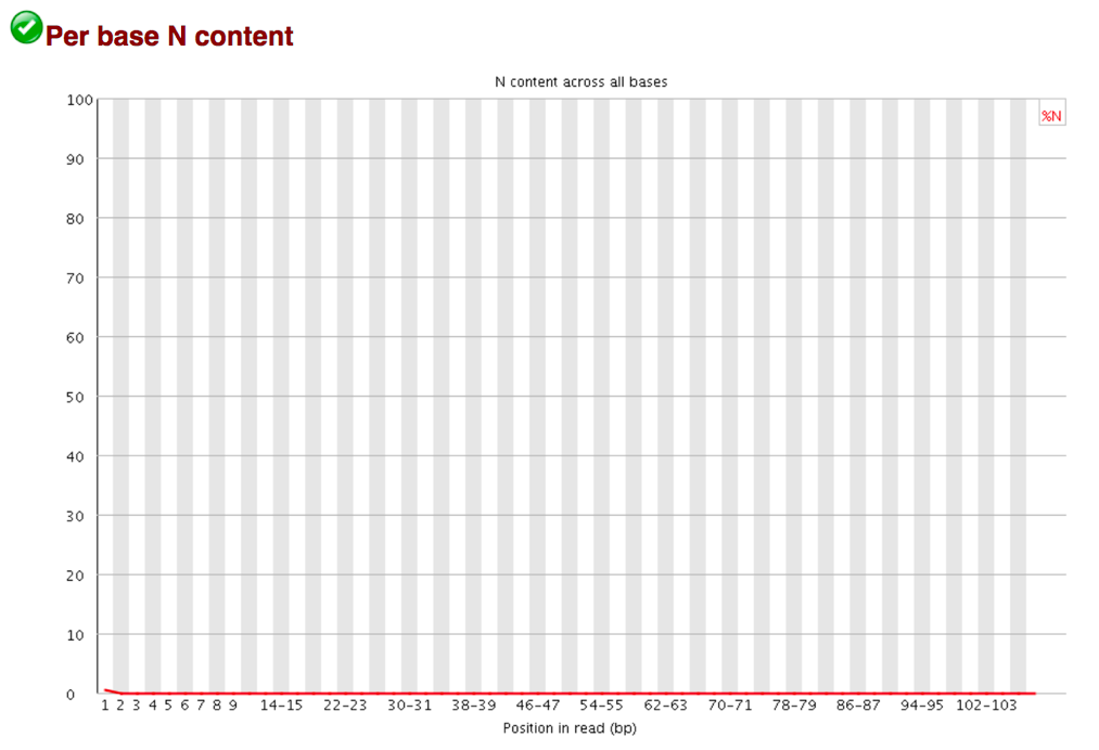
9. The Per Base N Content graphs shows the percent of bases at each position or bin with no base call, i.e. N.

1. You should never see any point where this curve rises noticeably above zero. If it does this indicates a problem occurred during the sequencing run.

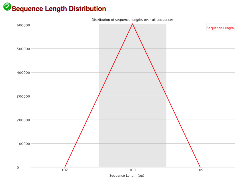
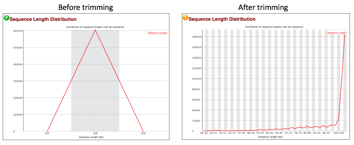
10. The Sequence Length Distribution module generates a graph showing the distribution of fragment sizes in the file which was analyzed.

1. Some high throughput sequencers generate sequence fragments of uniform length, but others can contain reads of wildly varying lengths. Even within uniform length libraries some pipelines will trim sequences to remove poor quality base calls from the end. In many cases this will produce a simple graph showing a peak only at one size, but for variable length FastQ files this will show the relative amounts of each different size of sequence fragment. This module will raise a warning if all sequences are not the same length, or if any of the sequences have zero length.

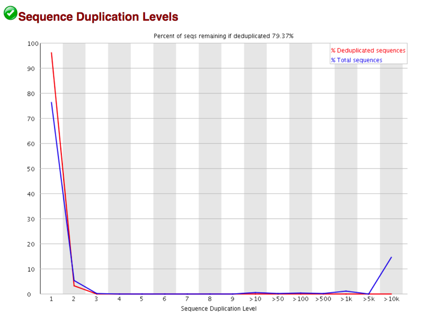
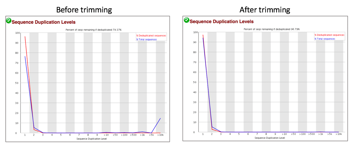
11. Sequence Duplication Levels Percentage of reads of a given sequence in the file which are present a given number of times in the file. (This is the blue line. The red line is more difficult to interpret.)

1. There are generally two sources of duplicate reads: PCR duplication in which library fragments have been over represented due to biased PCR enrichment or truly over represented sequences such as very abundant transcripts in an RNA-Seq library. The former is a concern because PCR duplicates misrepresent the true proportion of sequences in your starting material. The latter is an expected case and not of concern because it does faithfully represent your input. For whole genome shotgun data it is expected that nearly 100% of your reads will be unique (appearing only 1 time in the sequence data). This indicates a highly diverse library that was not over sequenced. If the sequencing output is extremely deep (e.g. > 100X the size of your genome) you will start to see some sequence duplication; this is inevitable as there are in theory only a finite number of completely unique sequence reads which can be obtained from any given input DNA sample.

2. When sequencing RNA there will be some very highly abundant transcripts and some lowly abundant. It is expected that duplicate reads will be observed for high abundance transcripts.

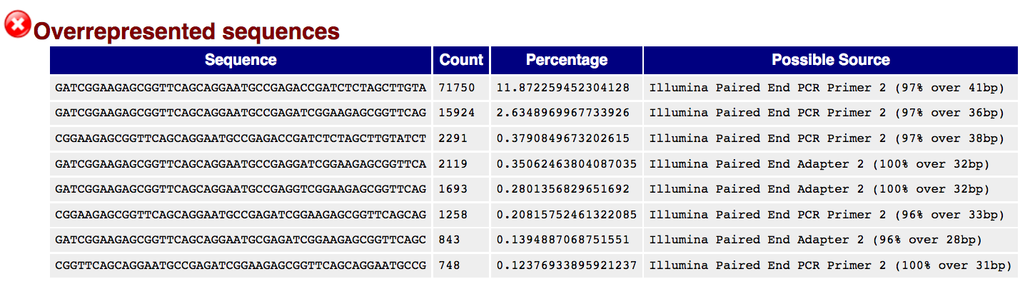
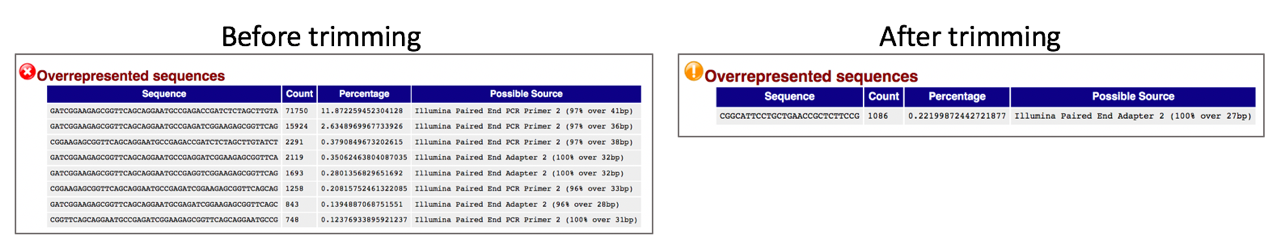
12. Overrepresented Sequences This shows a list of sequences which appear more than expected in the file. Only the first 50bp are considered. A sequence is considered overrepresented if it accounts for 0.1% of the total reads. Each overrepresented sequence is compared to a list of common contaminants to try to identify it.

1. In DNA-Seq data no single sequence should be present at a high enough frequency to be listed, though it is not unusual to see a small percentage of adapter reads.

2. For RNA-Seq data it is possible that there may be some transcripts that are so abundant that they register as overrepresented sequence.

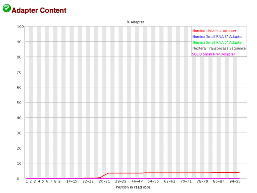
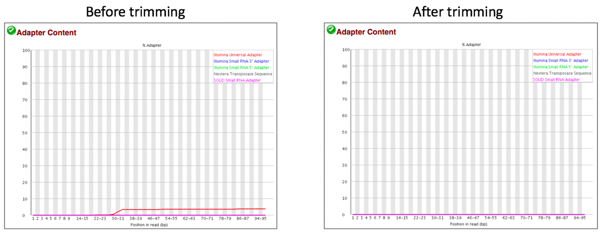
13. The Adapter Content shows a cumulative plot of the fraction of reads where the sequence library adapter sequence is identified at the indicated base position. Only adapters specific to the library type are searched. a. Ideally Illumina sequence data should not have any adapter sequence present, however when using long read lengths it is possible that some of the library inserts are shorter than the read length resulting in read-through to the adapter at the 3 end of the read. This is more likely to occur with RNA-Seq libraries where the distribution of library insert sizes is more varied and likely to include some short inserts.

Running Align

The Align function of the FastQC Utilities service aligns reads to genomes using Bowtie2[4, 5] to generate BAM files, saving unmapped reads, and generating SamStat[6] reports of the amount and quality of alignments. The Bowtie2 algorithm was downloaded from https://github.com/BenLangmead/bowtie2, and the SamStat algorithm from https://github.com/TimoLassmann/samstat.

Submitting the Align job

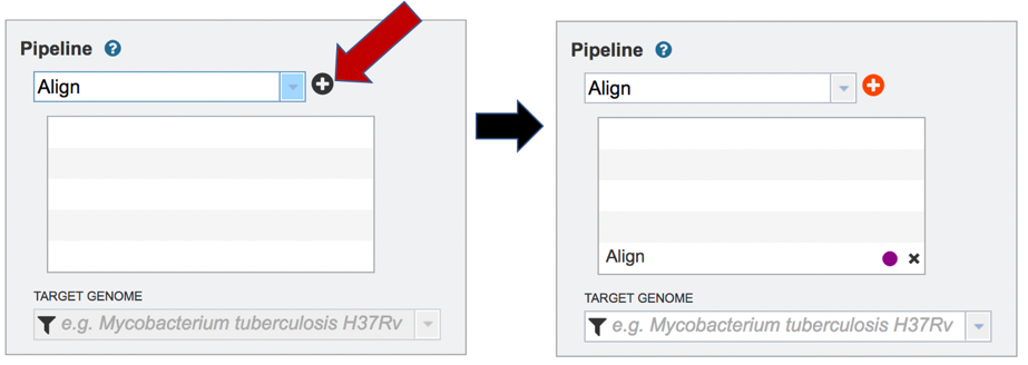
1. Clicking on Align in the drop-down box will move it into the text box. Click on the plus icon (+) at the end of the text box to move that pipeline into the selected service box below.

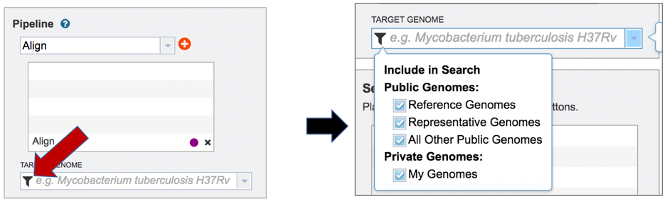
2. A genome to align the reads to must be selected. Any genome, private or public, available in PATRIC can be selected. Click on the filter icon at the left end of the text box underneath Target Genome to see the types of genomes that can be filtered on by clicking off the check boxes in front of unwanted genome types.

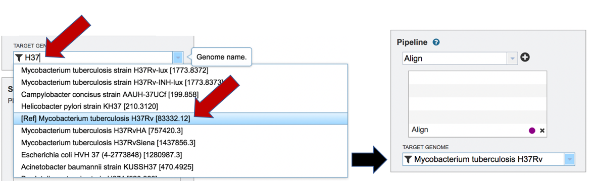
3. The name or genome ID of the desired target genome can be entered into the text box underneath Target Genome. Starting to type the strain name will show all genomes in PATRIC that match that combination, which will appear in the box below. Clicking on the name of the desired genome, once it appears, will autofill the name in the text box.

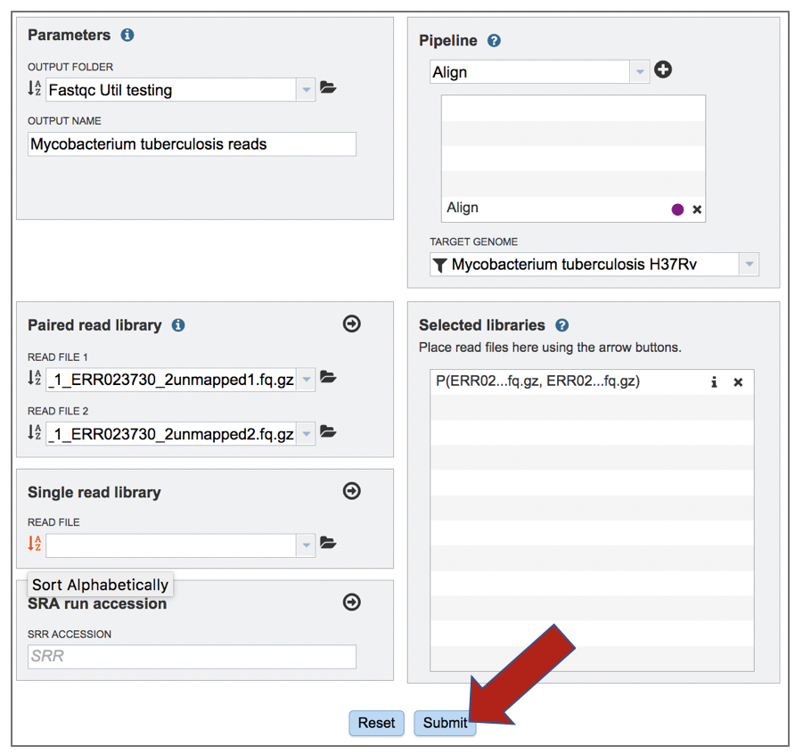
4. Once the Parameters, Algorithm, Target genome and Reads have been filled in or selected, the Submit button turns blue and the job will be submitted once clicked.

Viewing the Align job

1. A job that has been successfully completed can be viewed by clicking on the row and then clicking on the View icon in the vertical green bar.

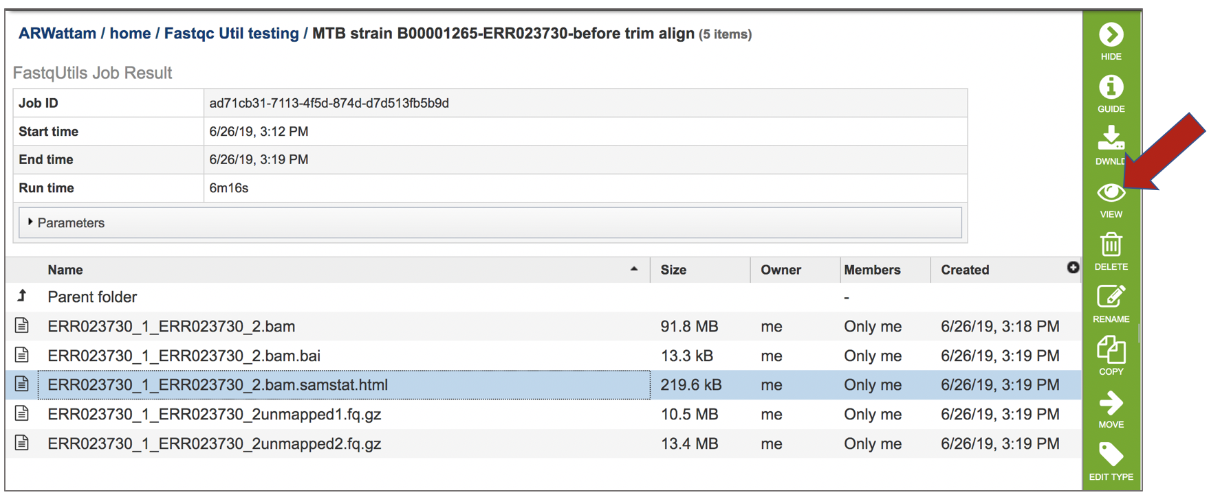
2. This will open the landing page for the selected job. The top box has the job ID number and gives pertinent information about the time it took to complete and the selected parameters. The lower table has four output files that include *.bam, *.bam.bai. *.html and *unmapped.fq.gz files.

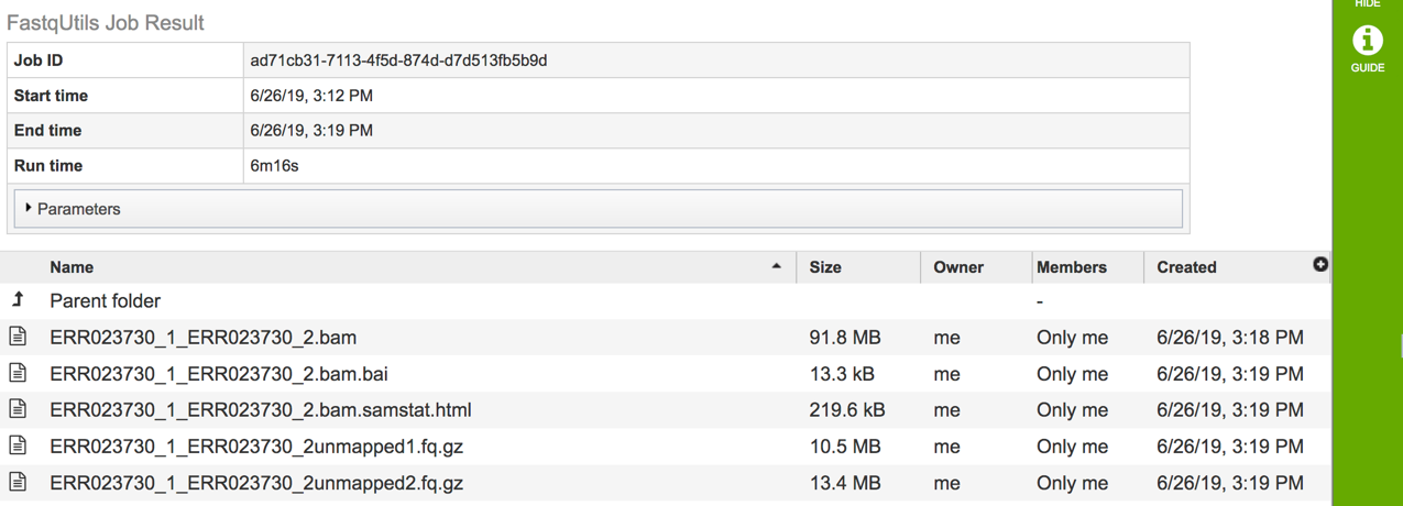
3. The *.bam and *bam.bai files can be downloaded. A BAM file (*.bam) is the compressed binary version of a SAM (Sequence Alignment/Map) file that is used to represent aligned sequences up to 128 Mb. BAM index files (*.bam.bai) provide an index of the corresponding BAM file.

4. If paired reads were submitted, the output files from the Align job will also provide a file that has all the reads from each read file that did not map to aligned to the target genome (*unmapped.fq.gz). If single reads were submitted, then only one *unmapped.fq.gz will be returned. These files can be downloaded.

5. To view the *bam.samstat.html file, click on the row that contains it and then on the View icon in the vertical green bar.

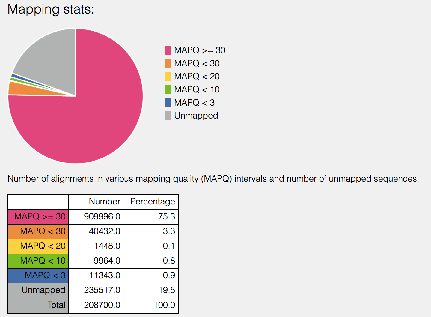
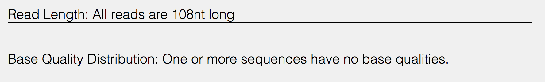
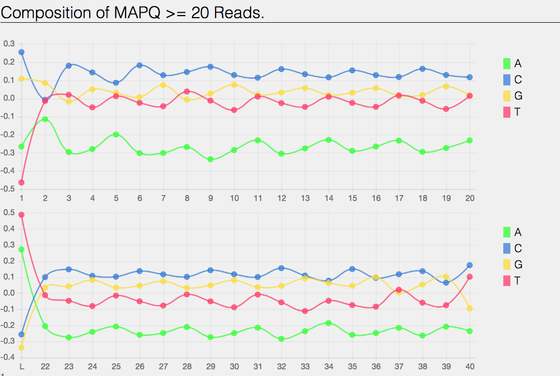
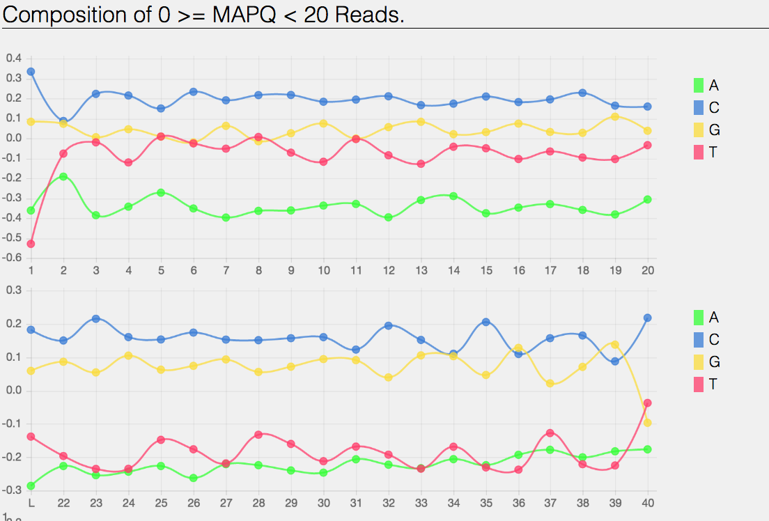
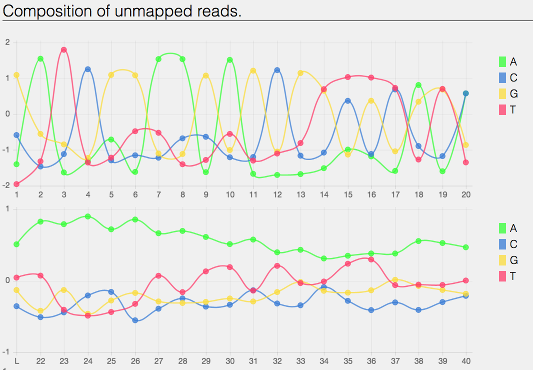
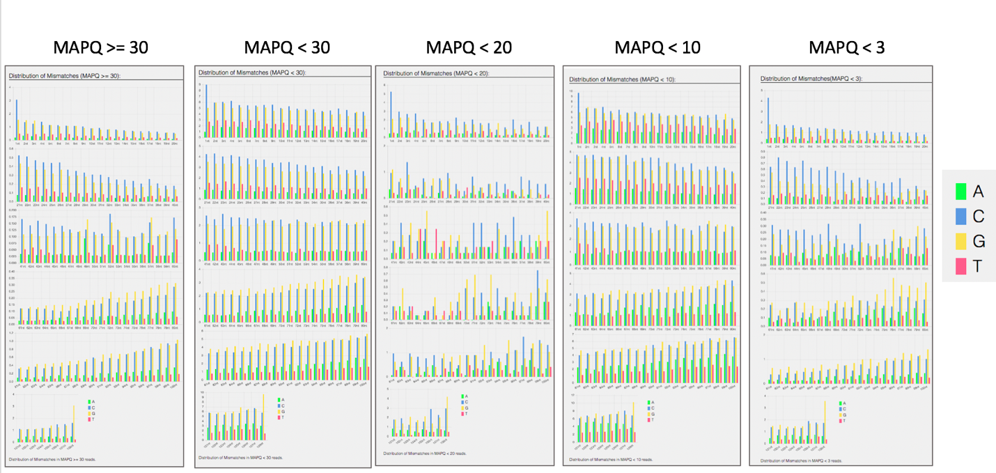
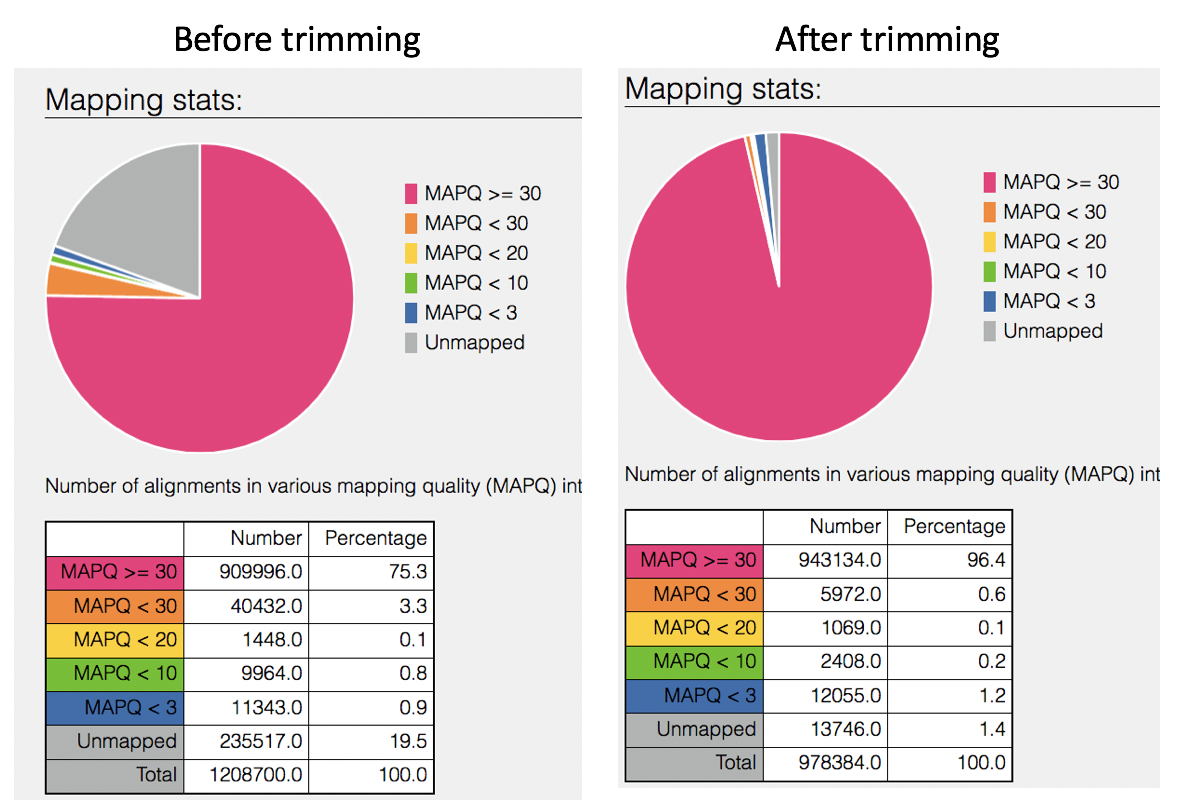
6. This will open the SAMStat report for the alignment job with the MAPQ statistics. The fifth column of a SAM file stores MAPping Quality (MAPQ) values. Mapping quality is the confidence that the read is correctly mapped to the genomic coordinates. For example, a read may be mapped to several genomic locations with almost a perfect match in all locations. In that case, alignment score will be high but mapping quality will be low. Reads falling in repetitive regions usually get very low mapping quality. Low quality means the observed read sequence is possibly wrong, and wrong sequence may lead to a wrong alignment.

7. Indication of the read length and the base quality distribution.

8. Composition of MAPping Quality (MAPQ) values that are greater or equal to 20 reads.

9. Composition of MAPping Quality (MAPQ) values that are greater than equal to 0 or less than 20 reads.

10. The composition of the unmapped reads.

11. Bar charts showing the distribution of mismatches along the read for alignments for each category of read quality.

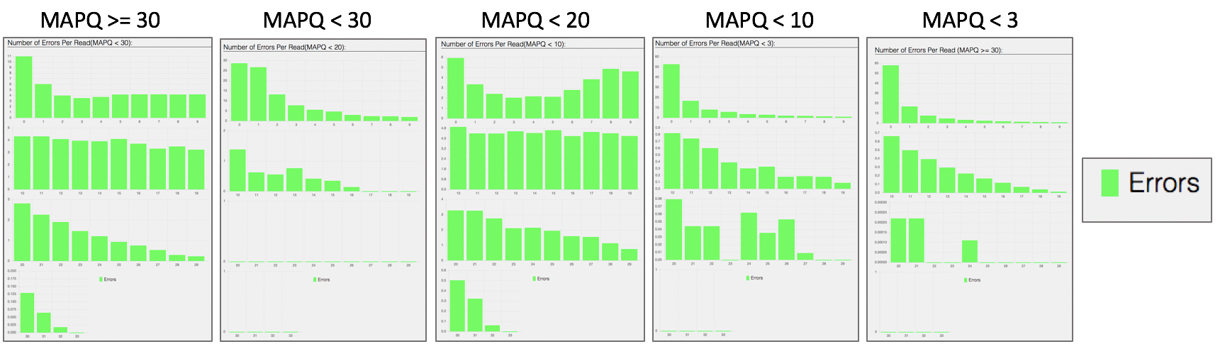
12. Bar plot showing the percentage of reads (y-axis) with 0, 1, 2 … errors (x axis) for MAPQ

Does trimming work?

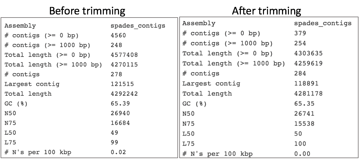
Reads from the same genome that were either trimmed or not, were run on the FASTQC, Align and Taxonomic Classification services in PATRIC to examine and compare results. Trimmed and untrimmed reads were also assembled using Spades[7]. Differences can be seen below.

1. Comparison of per base sequence quality in the FastQC report before and after trimming.

2. Comparison of per sequence quality scores before and after trimming.

3. Comparison of per sequence content before and after trimming.

4. Comparison of per sequence GC content before and after trimming.

5. Comparison of sequence length distribution before and after trimming.

6. Comparison of sequence distribution levels before and after trimming.

7. Comparison of overrepresented sequences before and after trimming.

8. Comparison of adaptor content before and after trimming.

9. Comparison of mapped reads from Align-FASTQC service results before and after trimming.

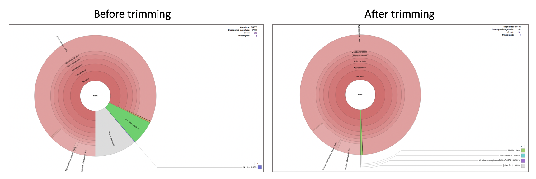
10. Comparison of Taxonomic Classification service results before and after trimming.

11. Comparison of assembly statistics generated by Spades before and after trimming.

References

1. Krueger, F., Trim Galore: a wrapper tool around Cutadapt and FastQC to consistently apply quality and adapter trimming to FastQ files, with some extra functionality for MspI-digested RRBS-type (Reduced Representation Bisufite-Seq) libraries. URL http://www.bioinformatics.babraham.ac.uk/projects/trim_galore/. (Date of access: 28/04/2016), 2012.

2. Martin, M., Cutadapt removes adapter sequences from high-throughput sequencing reads. EMBnet. journal, 2011. 17(1): p. 10-12.

3. Andrews, S., FastQC: a quality control tool for high throughput sequence data. 2010.

4. Langmead, B. and S.L. Salzberg, Fast gapped-read alignment with Bowtie 2. Nature methods, 2012. 9(4): p. 357.

5. Langmead, B., et al., Scaling read aligners to hundreds of threads on general-purpose processors. Bioinformatics, 2018. 35(3): p. 421-432.

6. Lassmann, T., Y. Hayashizaki, and C.O. Daub, SAMStat: monitoring biases in next generation sequencing data. Bioinformatics, 2010. 27(1): p. 130-131.

7. Bankevich, A., et al., SPAdes: a new genome assembly algorithm and its applications to single-cell sequencing. Journal of computational biology, 2012. 19(5): p. 455-477.